Conditional Formatting has been revamped in Excel 2007

Hi everyone

Ever wondered how you can get boring numerical data to be vibrant i.e. how can you make data like the one on the left hand to look like the one on the right hand side?

It is very simple and effective way to represent your data as mentioned above.

Please follow these steps:

• Highlight the cells that you wish to apply the conditional Formatting to


• On the Home Tab on the ribbon choose Condional Formatting and you will see various options available

• Chooose any relevant options. Following are some of the options:

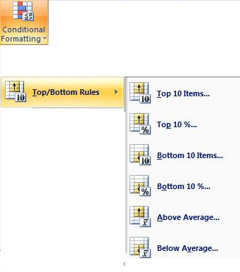
• You can change the settings of the Conditional formatting such as the your specific criteria, Icons or bar only, etc... by choosing Conditional Formatting and then Manage Rules... and chosing Edit Rule... button on the Manage Rules Dialog box


• If you wish to clear all teh Conditional Formatting Rules from specific cells then you can choose Conditional Formatting > Clear Rules > Clear rules from Selected cells or you can clear them from the entire sheet


• If you have applied various rules such as Data bar and Icon Sets and wish to delete one of the rules then you need to go to the manage rule dialog box and then select the rule and choose the Delete rule button.

If you found this to be helpful then please download your Free copy of the Excel Advanced Manual from www.mousetraining.co.uk/training-manuals/Excel2007adv.pdf

Cheers

Raj