Slicing Pivot Table without a knife

We all, who have been using Pivot tables, know that we can easily use the filter arrows to easily narrow the no. of records and type or records that we wish to see.

But wouldn't it be better if we didn't have to tick and untick every time we had to expand or narrow our selections. Slicers are the perfect answer to this type of situation. Slicers are floating

Please refer to the following figure where we have created a Pivot table for some staff of a fictitious company called ABC travels Ltd.

Lets see how Slicer can help in easily analyzing our data.

Step 1: Choose Insert and click on the Slicer button

Step 2: Choose the fields you would like for the slicing by putting a tick mark in front of them and then press OK button.

Once the Floating Slicers are on the screen you can easily choose the Dept or Region in our example to quickly slice the data you are looking for. If however, you are seeking multiple Depts or Regions then you can easily keep the CTRL button pressed and then click on the relevant selection on the slicers.

I would like to leave you with the last thought. From the two figures below which is easier and simpler to understand. Figure 1 with filters or the Figure 2 with the Slicers:

Figure 1:

Figure 2:

The beauty of Slicers is that like many other features of 2007 and 2010 you can instantly see the changes you make.

Hope this was helpful for you and that you will vist this website for other new features and tipand tricks!

Don't forget to download your free manuals for all the Microsoft office packages and many more applications from MTC website. Office 2010 manuals are on their way really soon!

Excel 2010 - Introduction of Sparklines

Have you ever tried to analyze data in rows or columns? The answer is Yes Of course!! But How long will it take you to see how well or unwell have you performed if you had twenty columns of data?


Those who are familiar with Conditional Formatting feature of Excel would appreciate the enhancement made in Excel 2007 comparatively to Excel 2003. Conditional formatting is very effective when you are looking at one instance of the data. But what if you are trying to see a Even better feature called Sparklines are introduced in Excel 2010


Sparklines are a great new addition in Excel 2010. These are effectively charts that can fit in a cell that allows you to easily analyze your data.


Following are some samples of Sparklines:

As you see from above figures how easily you can analyze data Monthly, Quarterly or Annually.

You can even highlight the High points or low points in different colours.


There are mainly three types of Sparklines: Line, Column and Win/Loss



To create spraklines please follow these steps:


Step 1: Select all the data you wish to create the sparklines for. In our example mentioned above the selected data would be A1: D5.


Step 2: Choose Insert on the ribbon. Select the sparkline of your choice i.e. Line, Column or Win/Loss




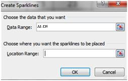
Step 3: In the Create Sparklines dialog box select the location range by selecting the cells where you would like to place the sparklines. In our examples above it will be E1: E5.

Step 4: Press OK

I hope you enjoyed this article and would strongly advice you to got to MTC website to get free downloadable course manuals for any of the office packages and other products. Please click Free Manuals Link to directly go to the free manuals section. Course manuals for Office 2010 will be available in the near future.

Conditional Formatting Entire Row

Conditional Formatting kills two birds with one stone! ( Not that I would like to be an efficient hunter)! First of all it makes your Spreadsheet look pretty and more importantly it provides you visual effect on which you can make instant decisions.

A time comes when you want the entire rows to change the colour based values on certain cells.

In our example above let's say that we want to make all the rows specific colours

1. Select the cells that you want to format.

2. In the menu bar, choose Format > Conditional Formatting...

3. In the Conditional Formatting dialog box, from the first drop-down list, choose Formula Is

4. In the text box, enter a formula that refers to the active cell in the selection. In this example, we selected A3:K27, and cell A3 is the active cell. So, in the formula, we'll refer to cell B3, because it's in the active row.

In this example, the formula is: =$E3<100000

In this example, we use an absolute reference to column E ($E), to ensure that the conditional formatting in all columns refers to the value in column E.

If we simply use a relative reference (E), the formula will be adjusted in each column, and won't work properly. Each cell will refer to the cell to its right, instead of refering to the cell in column E. Therefore we have to fix the Column E but not the Row 3 as we want that to change relatively.

5. Click the Format button. 6. In the Format Cells dialog box, select the formatting options that you want. You can choose Font format, Fill format and a Border format. 7. Click OK to close the Format Cells dialog box. 8. If you want to add more conditions, click the Add button, and repeat steps 3-8, for that condition. 9. Click OK, to close the Conditional Formatting dialog box. The final screen should look similar to the picture below.

I hope you benefited from this topic.

Please go to Mouse Training Website to get FREE Manuals for all the Office 2003 and 2007. Office 2010 is under construction and will be available in the near future.

Restrict data on cells for Invalid Data Using Data Validation!

Have you ever had a situation where you send a file or share a file with someone and they enter data that they weren't supposed to. Or may be enter too much data on a cell?

In Excel you have a feature called Data Validation that will help you in setting up the spreadsheet in such as way that users will not be able to enter any invalid data.

Looking at the following screen you can figure out that we need to restrict data on certain cells depending on the heading:

1. In the Initial field (Column) we want user to enter NO MORE than 1 character


2. In the Surname we want the data to be restricted to 15 characters only


3. DOB field shoudl only contain dates between 01/01/1948 and 31/01/98 only


4. No. of Laptops sold should be a Whole number and decimals should not be alowed

In order to restrict the cells with the above mentioned restrictions we need to highlight (select) the the relevant data.

• So we select A2: A19.


• From the menu bar we select Data > Validation...

• Click on the Drop down arrow for the Allow: and then choose Text Length
• From the Drop down of Data: choose Equal to
• In the length box type in 1 as we need users to ONLY enter one character in this field. Please note that there are many other options such as Greater than or equal to, Less than or Equal to , etc..
• Press OK.

I hope you get the idea how it works.

Following are the options that are available for various validations:

• Whole Number: This is if you wanted user to enter ONLY whole numbers and not Decimals. In our example it will be No. of Laptops field as you can not sell 1.5 laptops. Once you have mentioned whole number you can again set it to be between two values or greater than, less than, Equal to, etc...
• Decimal places: is where you want user to enter certain values meeting your specific criteria
• List: You can have drop down arrow appear in the cells that can show you various entries you would like to appear in the cells. You just have to enter the data separating them by a comma. In our example the Dept. field will have this type of data Validation.
• Date: This is for restricting cells to contain the dates meeting the specific requirements that you enter in the data validation dialog box.

You can also have specific messages appear on the screen if the user don't follow the guidelines that you set in the data validation dialog box.

For further details on this topic as well as other interesting topics please refer to the MOUSE Training link

Thank you for visiting and hope this topic was helpful!

Raj

Showing Millions in M on Cells

Ever wondered how you could have a figure such as 2,265,450 displayed as 2.26 M?

It is very simple to do.

1. Select all the cells that contain the values
2. Choose Format > Cells...
3. Ensure that you have Number tab selected
4. Choose Custom on the left hand side
5. Type the following in the Type: box (You can copy and paste it if you're feeling a bit lazy :)
[>=1000000]0.00,,"M"

And WALLAW! You get what you want! If you do want to see more numbers you can use the Increase and Decrease decimal buttons!

For downloading more tiops and trick and shortcust download FREE Manuals from http://www.mousetraining.co.uk/ms-office-training-manuals.html

Hope you have a nice day and thanks for visiting my blog!!

Conditional Formatting has been revamped in Excel 2007

Hi everyone

Ever wondered how you can get boring numerical data to be vibrant i.e. how can you make data like the one on the left hand to look like the one on the right hand side?

It is very simple and effective way to represent your data as mentioned above.

Please follow these steps:

• Highlight the cells that you wish to apply the conditional Formatting to


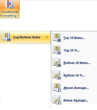
• On the Home Tab on the ribbon choose Condional Formatting and you will see various options available

• Chooose any relevant options. Following are some of the options:

• You can change the settings of the Conditional formatting such as the your specific criteria, Icons or bar only, etc... by choosing Conditional Formatting and then Manage Rules... and chosing Edit Rule... button on the Manage Rules Dialog box


• If you wish to clear all teh Conditional Formatting Rules from specific cells then you can choose Conditional Formatting > Clear Rules > Clear rules from Selected cells or you can clear them from the entire sheet


• If you have applied various rules such as Data bar and Icon Sets and wish to delete one of the rules then you need to go to the manage rule dialog box and then select the rule and choose the Delete rule button.

If you found this to be helpful then please download your Free copy of the Excel Advanced Manual from www.mousetraining.co.uk/training-manuals/Excel2007adv.pdf

Cheers

Raj

Excel Relative and Absolute Referencing

One of the main topics in MS Excel is understanding the difference between Relative referencing and Absolute Referencing. It seems to confuse many people who often copy/cut and paste cells that contain formulae and functions.

Hopefully this article should be able to clarify the differences.

Normally when you enter a formula in a cell and try to copy it to other cells the cells mysteriously start to change on the formulae and we start getting confused!

Lets see an Example

On the image above you can see that the AutoSum feature has been used on cell B7 to calculate the sum of Jan Sales. In order to calculate the sales for Feb and Mar that formula was simply copied and pasted using the Fill Handle ( the dark dot at the Bottom Right hand corner of the active cell).

The original formulae on cells B7 is: Sum(B2:B6) and when it was copied over to the other cells the cells updated to Sum C2:C6 and D2: D6 for C7 and D7 respectively. This is something Excel does automatically and is known as Relative Referencing.

Lets say that we decided to give 5% discount on the total of the product sales!

On the above image you'll see that the discount rate of 5% is on Cell I1 and the formula on Cell F2 is =E2*I1

If you tried to copy and paste the formula to other cells using the fill handle you will get the result as 0 in all the other cells!

The reason for this is because when you copy the formula the cells use the relative referencing and E2 change to E3, E4, E5 and E6 but I1 also change to I2, I3, I4 and I5. Therefore, we need to Fix the I1 so that when we copy the formula Every cell i.e. E3, E4, E5 and E6 should multiply with I1.

In Excel to do this we need to input $ signs. So if we modified the formula to be =E2*$I$1 and copy and paste it to the other cells the I1 will remain constant (Fixed) as seen on the next image:

To conclude I would like to state that sometimes we take Relative Referencing for Granted and assume that it will always work for us when ever we copy and paste cells that contain formulae but as seen above it did work for us when we did AutoSum but it didn't work at all when we tried to calculate the Discount! We had to fix I1 by entering formulae. So please be very careful before copying and pasting any formulae and functions.

If you found this post to be helpful you'll definitely find the FREE Training Manuals on Mouse Training Website.

I hope you'll come back to this for more Excel Help in the near future!